Why didn't you compare the KaKiOS catalog to the routine earthquake catalog produced by the SCEDC? Both report absolute locations so they should be comparable, no?
We did not consider the routine SCEDC locations because they are inconsistent in terms of depth. For many events, depth is not solved but rather fixed at constant values of 0, 1, 5.5, 6, 7 or 10 km (see Figure 1). This causes an arbitrary clustering at these depths and would thus bias the estimated multifractal spectrum and hinder subsequent comparisons. Removing all such events wouldn't be a solution since then we would have arbitrary gaps at these depths.
Furthermore, even if we wouldn't have locations with fixed depth, SCEDC does not report location uncertainties in their catalog, thus it would be difficult to interpret any observed scaling break in the multifractal analysis. In other words, earthquake locations are probability distributions and not points. Thus, it is problematic to compare distributions only in terms of means, in the absence of estimators for their variances.
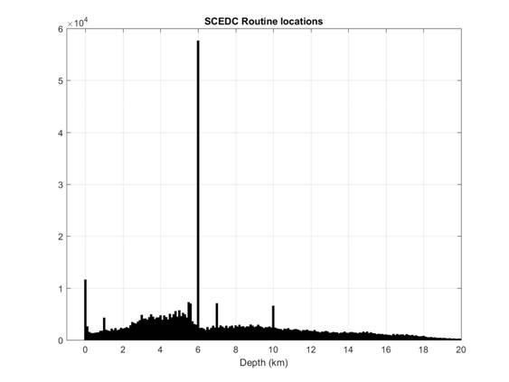
Figure 1: Depth histogram of routine SCEDC locations.
Are the KaKiOS location PDFs estimated assuming a constant velocity model, or do you also take into account uncertainties in the velocity structure?
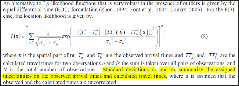
In common procedures (such as HypoEllipse, HypoInverse), hypocenters are estimated using a constant velocity model with no velocity modeling errors. In contrast, NonLinLoc uses a constant velocity model with a velocity modeling error expressed as a fraction of the travel time. In this study, the velocity modeling error has been obtained by analyzing the distribution of the station residuals using the 4 independent validation sets. Therefore, the shape and size of the location PDFs account for the velocity modeling uncertainty. This has been documented in Lomax et al. 2009 (see below) where "uncertainties in calculated travel times" refers to the uncertainties in velocity modeling.
Why do you consider absolute locations obtained using a minimum 1D velocity model superior to a catalog produced with double-difference, using a 3D velocity model. Can't it be that each approach has its own pros and cons for different uses?
This question suggests that earthquake catalogs are mere tools to be used by researchers and hence different applications might necessitate the existence of different tools (catalogs). We believe that a common terminology based on information and statistical theory is necessary to facilitate a fruitful debate. We maintain that earthquake catalogs are models used to fit/describe observational data. In the case of absolute locations, the data is the arrival times of seismic wave phases of interest (P, S, Pn, Pg, etc...): it constitutes an objective observation even if susceptible to human perception errors. Whereas, in the case of relative locations, the data is the differential times between sets of events determined by choices of minimum correlation coefficient, minimum neighboring distance and other triangulation parameters.
It is important to realize that, in the case of absolute locations, the data is not subject to change. However, in the case of relative locations, each earthquake is bound to change its relative location as new earthquakes are recorded, correlated and used in creating weighted bonds. In the case of Southern Californian seismicity, this conceptual difference has resulted in earthquake locations varying way beyond their initially reported location errors with each updated version of the relative location catalog (See Figure 1). In the light of this assessment and the additional caveats presented in the introduction of our paper, we believe that the choice of a catalog should be based on the consistency of data, resulting model and reported uncertainties. If one agrees that these criteria are relevant, then the choice becomes obvious.
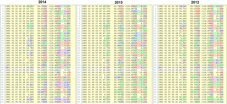
Figure 1: Text based comparison of the Southern California relative locations (first 40 entries) published in 2012, 2013 and 2014. Notice how ~30 year old events are being re-relocated (i.e. shifted) with each new version.
Tomographic studies for southern California show significant subsurface velocity variations throughout the crust. Given these observations, how valid is the use of a minimum 1-D model with station corrections?
Our use of a minimum 1-D model should not be misinterpreted as an assumption that there is not a significant 3-D variation in the southern Californian subsurface velocities. Our objective is to obtain a uniformly consistent seismicity catalog. Earthquakes are located by minimizing the difference between predicted and observed arrival times recorded at the stations. Thus, it follows that a model that can sufficiently represent the effective velocity averaged over the ray path from the source to the station should be sufficient for this task. Indeed, both northern and southern Californian seismic networks (and many networks worldwide) use 1-D velocity models for their routine earthquake locations. The resolution of 3-D velocity models varies significantly in the model volume due to varying ray coverage. This caveat can be tolerated for interpretation of structures; however it becomes problematic for routine location of seismicity, where uniform consistency is of importance for both well and poorly locatable events.
Furthermore, it has been well established that a minimum 1-D model constitutes the initial basis of any 3-D inversion due to the fact that it provides a consistent representation of the effective average velocities at depth. Thus, our use of a minimum 1-D model is not a choice but rather a requirement.
You keep refereing to KaKiOS as a "uniformly consistent" catalog. What do you mean by this, consistent for what?
The research that led us here started ~5 years ago. Our goal was (and still is) to apply likelihood based pattern recognition methods for the reconstruction of seismogenic faults. Unfortunately we found these methods, which are considered the state-of-the-art in many fields today, inapplicable to DD catalogs. This failure manifests itself in different analytical and computational forms but boils down to the violation of the notion of independent data. Therefore, the current work on absolute locations was motivated not by our curiosity or eagerness to push the state-of-the-art to the next level, but by sheer necessity. We cannot stress this enough: none of the DD relocated catalogs can be used to conduct an unbiased hypothesis test of an earthquake-to-earthquake interaction model. Most events are made dependent on each other through cross-correlation. This should be alarming for anybody who appreciates the importance of hypothesis testing, cross-validation etc... especially in seismology.
With this encompassing view in mind, our goal is "a uniformly consistent catalog" that would lend itself to the application of the basic scientific method: formulation and unbiased testing of hypotheses. We do not reject the existence of spatial subsurface velocity variations. Far from it, we use their observable surface expressions (local geology) to test and validate our velocity model. We do, however, note that in order to avoid producing local artifacts, a 3D model must be completely (volume wise) and equally well-resolved. The optimal model (in terms of uniformly consistent locations) for a region with non-regular 3D data distribution is a minimum 1D model with station delays to account for near-surface velocity variations. This min-1D model is well-resolved and complete in coverage with respect to the depth variations, which is a first order effect due the lithostatic pressure. Once this first order feature is well-resolved, local variations that become visible are recognized since they are quantitatively compatible regionally. Compare this with the formulation of double-difference where such local variations are exploited with assumptions (assuming a constant slowness vector for "sufficiently close events"). These exploitations lead to differences that cannot be consistent in the whole catalog (due to non-regular lateral coverage).
Isn't a 6-layer minimum 1-D model too simplistic? There is so much data available these days, 3-D models can be described at high resolution with large number of parameters.
For a general comparison, consider the Southern Californian section of the statewide 3D velocity model [Lin et al., 2010] (herein referred to as Lin2010). Notwithstanding the fact that the Lin2010 does not start from a minimum 1-D velocity model, and hence is susceptible to a biased convergence, the number of free parameters is an important consideration when comparing different models. Different aspects need to be considered too. We address this question from the following points of view:
1) Data: In our model, we use one training dataset and a total of 4 validation datasets that are used to constrain the velocities at different depths and the station correction. This amounts to a total of 10,387 earthquakes and 298,710 picks. Whereas, for Southern California, Lin2010 uses only 3,668 earthquakes with an average of 63 picks per event, yielding a total of 231,084 picks.
2) Data selection: Our selection criteria ensure uniform coverage and are based on a ranking according to both azimuthal gap and number of picks. The Lin2010 criterion selects the event only based on having the highest number of picks in its proximity. This results in a non-uniform areal coverage. Compare Figure 2 of this paper with Figure 2a of Lin et. al. 2010.
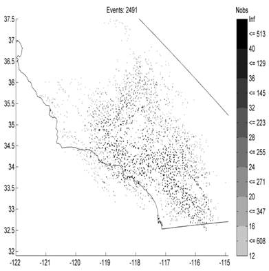
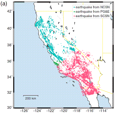
Figure 3: Spatial distributions of events used in this study (left) and Lin et al. 2010 (right).
3) Model complexities: The number of free parameters in the presented minimum 1-D velocity model is 13 (depth layers) + 436 (station delays) = 449. The Lin2010 model is a 3D grid with 9 depth layers, each sampled by a 61 x 66 grid at a resolution of 10km. To estimate the total number of free parameters in this model, we have to consider the fact that, due to the damping parameter in the inversion, the values at each grid node are correlated with their neighbors. To account for this correlation, we compute the vertical and horizontal autocorrelation for the velocities at each depth layer. The correlation length is the lag at which the autocorrelation first drops below zero. Thus, for each depth layer we can estimate the average correlation length in vertical and horizontal direction. Figure 4 shows the individual autocorrelation series at each depth level. Dividing the number of grid points at each depth layer by the product of the lateral correlation lengths, we estimate the total number of free parameters to be 428. Thus, we conclude that the complexity levels of our minimum 1-D model and the Lin2010 3-D model for Southern California are very similar.
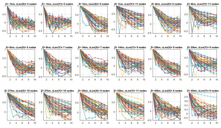
Figure 4: Autocorrelation curves for each depth layer (Z); cLen(X) and cLen(Y) indicate the average node at which the autocorrelation drops to zero.
4) Model performance and consistency: The average RMS value we obtain for our training and validation datasets is 0.18s. Lin2010 does not report an individual RMS value for Southern California, however their statewide RMS value is 0.32s. Even if the two models might be very similar in terms of their complexities, it is difficult to compare RMS values obtained from different datasets. It could be that our model provides a better fit or that our selection criteria have resulted in more well-locatable events. Hence we fail to see an obvious reason that would warrant the Lin2010 3D model to be preferred over our minimum 1D velocity model.
What if I still have questions?
Please contact your corresponding KaKiOS doctor